OSSE SWOT Filtering North Atlantic

SWOT karin error filtering (2022a)

A challenge on the SWOT Karin instrumental error filtering organised by Datlas, IMT Altlantique and CLS.

Context & Motivation

The two-dimensional sea level SWOT products are very much expected to be a game changer in many oceanographic applications which will make them an unprecedented L3 product to be distributed. The row SWOT data will however be contaminated by instrumental and geophysical errors (Gauthier et al., 2016; Peral and Esteban-Fernandez, 2018). In order to be able to observe front, mesoscale and sub-mesoscale features, the SWOT data will require specific processing. Also, these errors are expected to strongly pollute the first and second derivatives of the SSH data which are used for the computation of geostrophic currents and vorticity. Hence, being able to remove the SWOT errors will be of significant importance to recover information on 2D surface currents and vertical mixing.

The SWOT errors are expected to generate noises that are both correlated on the swath and spatially uncorrelated. Several past efforts have already investigated methods to remove or reduce the correlated noises from the SWOT data using prior knowledge on the ocean state (e.g. Metref et al., 2019, see Figure 2.4.A), calibration from independent Nadir altimeter data (e.g. Febvre et al., 2021, see Figure 2.4.B) or cross-calibration from SWOT data themselves (on-going CNES-DUACS studies). And other efforts focused on reducing the uncorrelated data (Gomez-Navarro et al., 2018, 2020; Febvre et al., 2021). Yet, so far, no rigorous intercomparison between the recently developed methods has been undertaken and it seems difficult, to this day, to outline the benefits and limitations of favoring one error reduction method from another.

It is important to mention that the SWOT science requirement for uncorrelated noise measurement error specifies that KaRin must resolve SSH on wavelength scales up to 15 km based on the 68th percentile of the global wavenumber distribution.

The goal of this Filtering SWOT data challenge is to provide a platform to investigate the most appropriate filtering methods to reduce the uncorrelated instrumental (KaRIn) noise from the SWOT data.

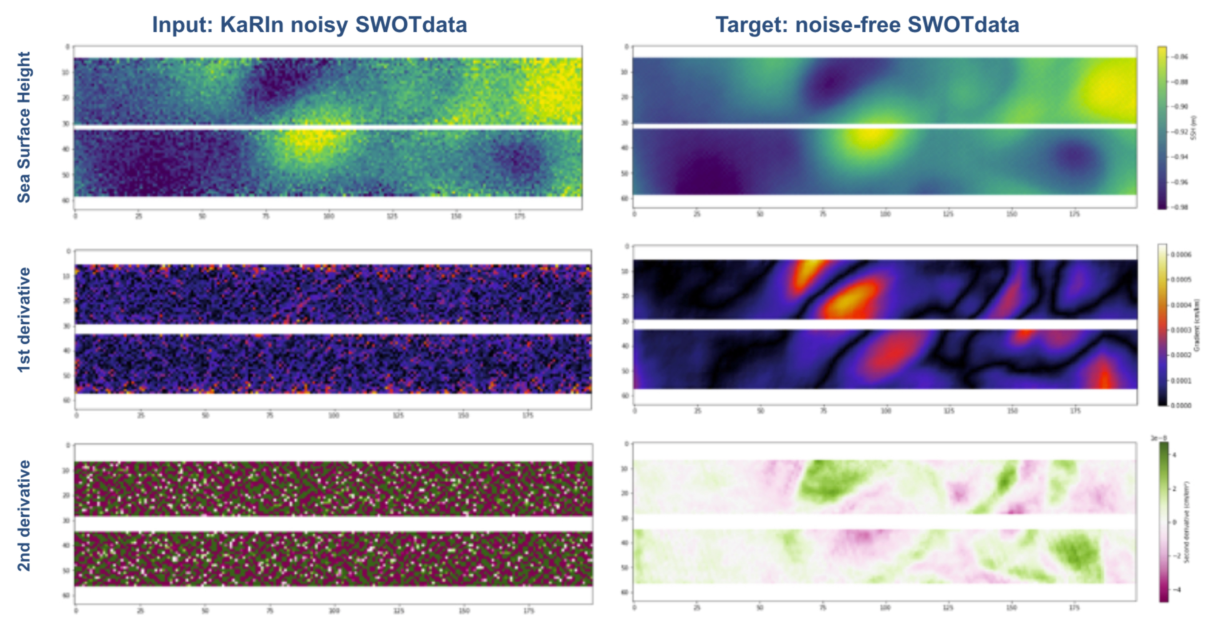
In practice, the data challenge is in the form of an Observing System Simulation Experiment (OSSE) considering a realistic ocean model simulation (eNATL60) as the true ocean state. The SWOT simulator (Gauthier et al., 2016) was then used to create realistic SWOT data with and without instrumental noise. Then, various filtering methods are tested and compared to the true ocean state.

This data challenge is part of the Sea Level Innovations and Collaborative Intercomparisons for the Next-Generation products (SLICING) project, funded by Copernicus Marine Service Evolution (21036-COP-INNO SCI).

Data sequence and use

The data challenge is in the form of an Observing System Simulation Experiment (OSSE) considering a realistic ocean model simulation, the NEMO high resolution North Atlantic simulation eNATL60, as the true ocean state. The SWOT simulator (Gauthier et al., 2016) was then used to create realistic SWOT data with and without instrumental noise.

The experiment is performed over one SWOT orbital cycle (cycle 13) which contains 270 passes. All other cycles are available to tune or train the filters.

The noisy SWOT data to filter (the inputs: ssh_karin) and their equivalent noise-free SWOT data for evaluation (the targets: ssh_true) are hosted and available for download on the MEOM opendap server: see Download the data section below. In no way the targets that are available during the evaluation period should be used in the filtering process (including for tuning the filter).

Fig.: Example of SWOT noisy input products and target fields to be restore with a filtering method (picture from A. Treboutte)

Data format

The data are hosted on the opendap: ocean-data-challenges/2022a_SWOT_karin_error_filtering/.

Data challenge data

The data needed for the DC are presented with the following directory structure:

.
|-- dc_inputs
|   |-- input_ssh_karin_013_*.nc

To start out download the dataset from the temporary data server, use:

!wget https://ige-meom-opendap.univ-grenoble-alpes.fr/thredds/fileServer/meomopendap/extract/ocean-data-challenges/2022a_SWOT_karin_error_filtering/dc_inputs.tar.gz

and then uncompress the files using tar -xvf <file>.tar.gz. You may also use ftp, rsync or curlto donwload the data. The inputs are stored in the variable ssh_karin and the targets are stored in the variable *ssh_true.

Extra training data

If necessary a dataset for training purposes is available and structured as follows:

. 
|--  

and can be downloaded using:

Leaderboard

Method	Field	µ(RMSE global)	µ(RMSE coastal)	µ(RMSE offshore lowvar)	µ(RMSE offshore highvar)	λ(SNR1) [km]	Reference
NO FILTER	Sea Surface Height [m]	0.013	0.012	0.013	0.014	44.5	demo_benchmark_MEDIAN.ipynb
NO FILTER	Geostrophic current [m.s^-1]	0.917	0.801	1.073	0.545	687.5	demo_benchmark_MEDIAN.ipynb
NO FILTER	Relative vorticity []	18.733	14.396	22.559	4.719	>=1000	demo_benchmark_MEDIAN.ipynb

MEDIAN	Sea Surface Height [m]	0.028	0.045	0.004	0.008	23.3	demo_benchmark_MEDIAN.ipynb
MEDIAN	Geostrophic current [m.s^-1]	0.203	0.311	0.085	0.117	28.7	demo_benchmark_MEDIAN.ipynb
MEDIAN	Relative vorticity []	1.846	2.666	1.247	0.619	>=1000	demo_benchmark_MEDIAN.ipynb

GOMEZ	Sea Surface Height [m]	0.025	0.040	0.002	0.003	21.5	demo_benchmark_GOMEZ.ipynb
GOMEZ	Geostrophic current [m.s^-1]	0.202	0.323	0.064	0.056	23.4	demo_benchmark_GOMEZ.ipynb
GOMEZ	Relative vorticity []	1.671	2.569	0.871	0.329	812.3	demo_benchmark_GOMEZ.ipynb

CNN	Sea Surface Height [m]	0.002	0.002	0.002	0.003	10.5	demo_benchmark_CNN.ipynb
CNN	Geostrophic current [m.s^-1]	0.055	0.068	0.043	0.051	9.4	demo_benchmark_CNN.ipynb
CNN	Relative vorticity []	0.637	0.881	0.475	0.303	15.4	demo_benchmark_CNN.ipynb

GOMEZ_V2	Sea Surface Height [m]	0.002	0.0026	0.002	0.003	14.8	no notebook available, spat. variable param
GOMEZ_V2	Geostrophic current [m.s^-1]	0.056	0.065	0.050	0.057	12.5	no notebook available, spat. variable param
GOMEZ_V2	Relative vorticity []	0.65	0.882	0.504	0.321	26.6	no notebook available, spat. variable param

with:

µ(RMSE global): averaged root-mean square error over the full domain

µ(RMSE coastal): averaged root-mean square error in coastal region (distance < 200km from coastine)

µ(RMSE offshore lowvar): averaged root-mean square error in offshore (distance > 200km from coastine) and low variability regions ( variance < 200cm²)

µ(RMSE offshore highvar): averaged root-mean square error in offshore (distance > 200km from coastine) and high variability regions ( variance > 200cm²)

λ(SNR1): spatial wavelength where SNR=1

Installation

:computer: How to get started ?

Clone the data challenge repo:

git clone https://github.com/ocean-data-challenges/2022a_SWOT_karin_error_filtering.git

create the data challenge conda environment, named env-dc-swot-filtering, by running the following command:

conda env create --file=environment.yml

and activate it with:

conda activate env-dc-swot-filtering

then add it to the available kernels for jupyter to see:

ipython kernel install --name "env-dc-swot-filtering" --user

You’re now good to go !

Check out the quickstart

Download the data

Acknowledgement

This data challenge was created as part of the Service Evolution CMEMS project: SLICING, in collaboration with Datlas, CLS, IMT-Atlantique.

The structure of this data challenge was to a large extent inspired by the ocean-data-challenges created for the BOOST-SWOT ANR project.

The experiment proposed and the illustrative figures contained in this data challenge are based on an internal study conducted at CLS by Anaelle Treboutte & Pierre Prandi